4.1.5 Analyse des cartes
Les cartes forêt/non-forêt nettoyées de 1987 à 2018 sont utilisées pour créer des cartes des changements forestiers. En utilisant la fonction fc() les pixels qui passent d’une situation “non-forêt” ou “régénération potentielle” à “régénération” sont enregistrés comme gains de surface forestière dans l’année correspondante, les pixels qui passent d’une situation “forêt” ou “régénération” à “non-forêt” sont enregistrés comme perte de surface forestière. Sur cette base, pour chaque année disponible dans la série, une compilation des surfaces forestières, de la surface régénérée et de la régénération potentielle, ainsi que des gains et pertes de forêts dans la période précédente est effectuée.
Le tableau de la superficie forestière sert à son tour de base pour déterminer les changements annuelles de la surface forestière sur différentes périodes de temps à l’aide de la fonction fcc(). En plus des changements annuelles absolues, les taux de changement correspondants sont calculés selon la formule suivante : \(r = (1/(t2 - t1)) \times ln(A2/A1)\) (Puyravaud, 2003).
La fonction plot.fc() affiche graphiquement le tableau des surfaces forestières et montre comment la surface forestière et la régénération se développent. La fonction plot.fcc() crée un diagramme en barres des gains et des pertes annuelles de la surface forestières sur certaines périodes de temps.
Enfin, des cartes de la perte de forêts, de la régénération potentielle et de la régénération sont créées, avec les années de changement observées comme valeurs de pixel.
Example
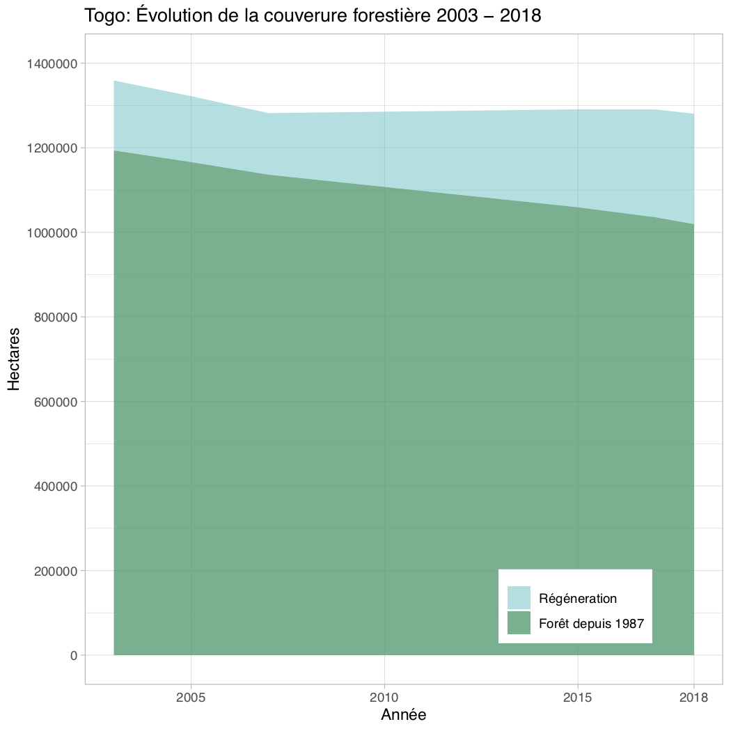
Tableau des superfaces forestières pour le Togo La surface forestière initiale (existant depuis 1987), la superficie forestière secondaire (régénérée depuis 1987), la surface de la régénération potentielle (< 10 ans) et la déforestation et l’accroissement enregistrés dans la période précédente. Tous les chiffres sont exprimés en hectares.
| Année | Surface f. totale | Surface f. initiale | Surface f. secondaire | Régén. potentielle | Pertes surface f. | Gains surface f. |
|---|---|---|---|---|---|---|
| 1987 | 1’265’377 | 1’265’377 | 0 | 133’038 | — | — |
| 2003 | 1’359’051 | 1’193’731 | 165’320 | 90’972 | -71’646 | 165’320 |
| 2005 | 1’321’963 | 1’166’156 | 155’807 | 122’718 | -37’088 | 0 |
| 2007 | 1’281’909 | 1’136’373 | 145’536 | 161’787 | -40’154 | 101 |
| 2015 | 1’290’948 | 1’059’301 | 231’647 | 156’237 | -99’560 | 108’600 |
| 2017 | 1’290’615 | 1’035’724 | 254’891 | 169’171 | -39’503 | 39’170 |
| 2018 | 1’280’513 | 1’019’489 | 261’024 | 188’715 | -27’027 | 16’925 |
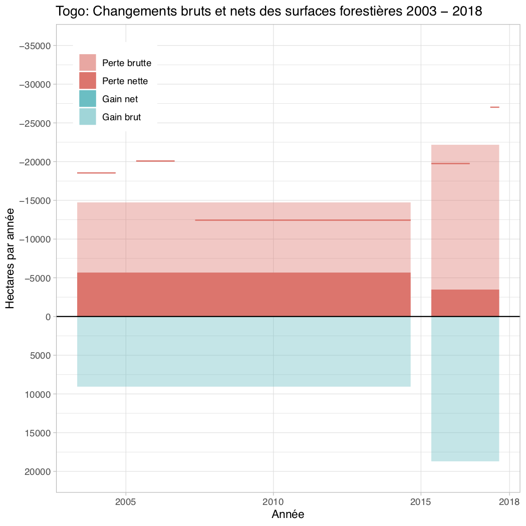
Changement annuelle de la superficie forestière au Togo, pour 2003 – 2015, 2015 – 2018 et toute la période 2003 – 2018, montrant les pertes et les gains brutes des forêts, et le changement net de la surface forestière en hectares par an et les taux correspondants en %/an.
| Période | Pertes (ha/an) | Gains (ha/an) | Ch. net (ha/an) | Pertes (%/an) | Gains (%/an) | Ch. net (%/an) |
|---|---|---|---|---|---|---|
| 2003 – 2015 | -14’734 | 9’058 | -5’675 | -1.2 | 0.6 | -0.4 |
| 2015 – 2018 | -22’177 | 18’699 | -3’478 | -1.8 | 1.4 | -0.3 |
| 2003 – 2018 | -16’222 | 10’986 | -5’236 | -1.3 | 0.8 | -0.4 |
Changement de la surface forestière du Togo 2003 – 2018 Changement de la superficie forestière (à gauche) ansi que les gains et les pertes annuelles pour les périodes 2003 – 2015 et 2015 – 2018 (à droite).
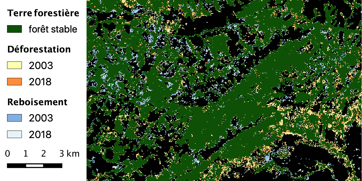
Complexité de l’évolution de la superficie forestière en prenant l’exemple d’une petite partie de la région des Plateaux. Pertes de forêts 2003 – 2018 (jaune à orange) et croissance des forêts au cours de la même période (bleu à blanc). Le fond noir est non-forêt sur toute la période.
MCF/05_analyse-fc-maps.R
##########################################################################
# NERF_Togo/FCC/8_analyse-fc-maps.R: analyze clean forest cover maps
# ------------------------------------------------------------------------
# Bern University of Applied Sciences
# Oliver Gardi, <oliver.gardi@bfh.ch>
# 20 May 2019

COV.FC         <- 30

# Function for building forest cover table ---------------------------------

fc <- function(map, aoi=NULL) {

  if(!is.null(aoi)) map <- mask(crop(map, aoi), aoi)

  # convert non-forest to 0
  # potential regeneration to 1
  # regeneration to 2
  # forest to 3

  tab.fc <- map[]
  tab.fc[tab.fc == 3] <- 0
  tab.fc[tab.fc == 1] <- 3
  tab.fc[tab.fc == 2] <- 1


  for(i in 2:ncol(tab.fc)) {
    tab.fc[!is.na(tab.fc[,i]) & tab.fc[,i] == 3 & !is.na(tab.fc[,i-1]) & tab.fc[,i-1] < 3, i] <- 2  # mark as regeneration when it was non-forest or regeneration before
  }

  tab.fcc <- tab.fc[,1:ncol(tab.fc)-1]
  tab.fcc[] <- 0
  for(i in 1:ncol(tab.fcc)) {
    tab.fcc[tab.fc[,i] <= 1 & tab.fc[,i+1] >= 2, i]   <- 1           # mark forest gain
    tab.fcc[tab.fc[,i] >= 2 & tab.fc[,i+1] <= 1, i]   <- 2           # mark forest loss
  }

  dates <- as.numeric(substr(names(map), 2, 5))

  fc <- data.frame(year     = dates,
                   initi.ha = colSums(tab.fc==3, na.rm=TRUE) * 30^2/10000,
                   secon.ha = colSums(tab.fc==2, na.rm=TRUE) * 30^2/10000,
                   poten.ha = colSums(tab.fc==1, na.rm=TRUE) * 30^2/10000)

  fc$total.ha <-   fc$initi.ha + fc$secon.ha
  fc$defor.ha <-   -c(colSums(tab.fcc==2, na.rm=TRUE) * 30^2/10000, NA)
  fc$regen.ha <-    c(colSums(tab.fcc==1, na.rm=TRUE) * 30^2/10000, NA)

  return(fc)
}

fcc <- function(fc.tab, years=fc.tab$year) {

  for(i in 1:(length(years)-1)) {
    fc.tab$defor.ha.yr[fc.tab$year==years[i]] <- sum(fc.tab$defor.ha[fc.tab$year >= years[i] & fc.tab$year < years[i+1]])/(years[i+1]-years[i])
    fc.tab$regen.ha.yr[fc.tab$year==years[i]] <- sum(fc.tab$regen.ha[fc.tab$year >= years[i] & fc.tab$year < years[i+1]])/(years[i+1]-years[i])
    fc.tab$netch.ha.yr[fc.tab$year==years[i]] <- fc.tab$defor.ha.yr[fc.tab$year==years[i]] + fc.tab$regen.ha.yr[fc.tab$year==years[i]]

    fc.tab$defor.pc.yr[fc.tab$year==years[i]] <- round(100 * 1/(years[i+1]-years[i]) * log((fc.tab$total.ha[fc.tab$year==years[i+1]] - sum(fc.tab$regen.ha[fc.tab$year >= years[i] & fc.tab$year < years[i+1]]))/fc.tab$total.ha[fc.tab$year==years[i]]), 3)
    fc.tab$regen.pc.yr[fc.tab$year==years[i]] <- round(100 * 1/(years[i+1]-years[i]) * log((fc.tab$total.ha[fc.tab$year==years[i+1]] - sum(fc.tab$defor.ha[fc.tab$year >= years[i] & fc.tab$year < years[i+1]]))/fc.tab$total.ha[fc.tab$year==years[i]]), 3)
    fc.tab$netch.pc.yr[fc.tab$year==years[i]] <- round(100 * 1/(years[i+1]-years[i]) * log(fc.tab$total.ha[fc.tab$year==years[i+1]]/fc.tab$total.ha[fc.tab$year==years[i]]), 3)
  }

  return(fc.tab)
}

# Function for plotting evolution of forest cover -----------------------------------------

plot.fc <- function(fc, zone, filename=NULL) {

  if(zone=="TGO") {
    title    <- "Togo: Évolution de la couverure forestière 2003 - 2018"
    ylim     <- c(0, 1400000)
    ybreaks  <- seq(0, 1400000, 200000)
    ymbreaks <- seq(0, 1400000, 100000)
  } else {
    title    <- paste0(zone, ": Évolution de la couverure forestière 2003 - 2018")
    ylim     <- c(0, 500000)
    ybreaks  <- seq(0, 500000, 100000)
    ymbreaks <- seq(0, 500000, 50000)
  }

  if(!is.null(filename)) pdf(filename)

  print(
    fc %>%  gather(variable, value, secon.ha, initi.ha) %>%
      ggplot(aes(x = year, y=value, fill=variable)) +
      geom_area(position=position_stack(reverse=TRUE)) +
      scale_fill_manual(name = NULL, breaks=c("secon.ha", "initi.ha"), values=c(alpha("#009E73", 0.8), alpha("#00BFC4", 0.5)), labels=c("Régéneration", "Forêt depuis 1987")) +
      xlab("Année") + ylab("Hectares") + ggtitle(title) +
      scale_x_continuous(minor_breaks = NULL, breaks=c(1991, 2000, 2005, 2010, 2015, 2018)) +
      scale_y_continuous(breaks=ybreaks, minor_breaks = ymbreaks) + coord_cartesian(ylim=ylim) +
      theme_light() + theme(legend.position=c(0.6,0.2), legend.box = "horizontal", legend.justification=c(-0.2,1.2))
  )

  if(!is.null(filename)) dev.off()
}

# Function for plotting forest cover change -----------------------------------

plot.fcc <- function(fc, zone=NULL, breaks=NULL, filename=NULL) {

  my.fcc <- fcc(fc)
  fcc.breaks <- my.fcc

  if(!is.null(breaks)) fcc.breaks <- fcc(fc, breaks)[fc$year %in% breaks,]

  my.fcc$period <- c(my.fcc$year[2:nrow(my.fcc)] - my.fcc$year[1:(nrow(my.fcc)-1)], NA)
  my.fcc$center <- my.fcc$year + my.fcc$period/2

  fcc.breaks$period <- c(fcc.breaks$year[2:nrow(fcc.breaks)] - fcc.breaks$year[1:(nrow(fcc.breaks)-1)], NA)
  fcc.breaks$center <- fcc.breaks$year + fcc.breaks$period/2


  if(zone=="TGO") {
    title    <- "Togo: Changements bruts et nets des surfaces forestières 2003 - 2018"
    ylim     <- c(-35000, 20000)
    ybreaks  <- seq(-35000, 20000, 5000)
    ymbreaks <- seq(-35000, 20000, 2500)
  } else {
    title    <- paste0(zone, ": Changements bruts et nets des surfaces forestières 2003 - 2018")
    ylim     <- c(-15000, 10000)
    ybreaks  <- seq(-15000, 10000, 5000)
    ymbreaks <- seq(-15000, 10000, 2500)
  }


  if(!is.null(filename)) pdf(filename)

  fcc.breaks$netdefor.ha.yr <- fcc.breaks$netch.ha.yr
  fcc.breaks$netdefor.ha.yr[fcc.breaks$netdefor.ha.yr > 0] <- 0
  fcc.breaks$netregen.ha.yr <- fcc.breaks$netch.ha.yr
  fcc.breaks$netregen.ha.yr[fcc.breaks$netregen.ha.yr < 0] <- 0

  print(
    fcc.breaks[-nrow(fcc.breaks),] %>% gather(variable, value, defor.ha.yr, regen.ha.yr, netdefor.ha.yr, netregen.ha.yr) %>%
      ggplot(aes(y=value, x = center, width=period-0.7)) +
      geom_bar(data=. %>% filter(variable %in% c("defor.ha.yr", "regen.ha.yr")), aes(fill=variable), stat = "identity") +
      geom_bar(data=. %>% filter(variable %in% c("netdefor.ha.yr", "netregen.ha.yr")), aes(fill=variable), stat = "identity") +
      geom_errorbar(data=my.fcc[1:5,], aes(x=center, y=NULL, ymax=defor.ha.yr, ymin=defor.ha.yr, width=period-0.7), colour=alpha("#F8766D", 1)) +
      geom_hline(aes(yintercept=0)) +
      scale_fill_manual(name = NULL, breaks = c("defor.ha.yr", "netdefor.ha.yr", "netregen.ha.yr", "regen.ha.yr"), values=c("regen.ha.yr" = alpha("#00BFC4", 0.4), "netregen.ha.yr" = "#00BFC4", "netdefor.ha.yr" = "#F8766D", "defor.ha.yr" = alpha("#F8766D", 0.4)), labels=c("Perte brutte", "Perte nette", "Gain net", "Gain brut")) +
      xlab("Année") + ylab("Hectares par année") + ggtitle(title) +
      scale_x_continuous(minor_breaks = NULL, breaks=c(1991, 2000, 2005, 2010, 2015, 2018)) +
      scale_y_reverse(breaks=ybreaks, minor_breaks = ymbreaks) + coord_cartesian(ylim=ylim) +
      theme_light() + theme(legend.position=c(0,1), legend.box = "horizontal", legend.justification=c(-0.2,1.2))
  )

  if(!is.null(filename)) dev.off()
}


# DO THE WORK ##############################

# Load and rename forest-cover maps ----------------------------

maps <- stack(dir(paste0(FCC.CLN.DIR, "/FC", COV.FC, "/TGO"), pattern = "cf.tif", full.names = TRUE))
names(maps) <- paste0("X", substr(names(maps), 5, 8))

# Create forest cover tables for different periods ------------------------------------

fc.all      <- fc(maps)
write.csv(fc.all, paste0(FCC.RES.DIR, "/TGO/TGO_fc.csv"), row.names=FALSE)

fc.all <- read.csv(paste0(FCC.RES.DIR, "/TGO/TGO_fc.csv"))

fc.cln <- fc.all
fc.cln <- fc.cln[!fc.cln$year %in% c(1987, 1991, 2000), ]

fcc(fc.cln)
fcc(fc.cln, c(2003, 2018))
fcc(fc.cln, c(2003, 2015, 2017, 2018))

write.xlsx(list("Total" = fcc(fc.cln)), file = paste0(FCC.RES.DIR, "/TGO/TGO_fcc-all-dates.xlsx"))
write.xlsx(list("Total" = fcc(fc.cln, c(2003, 2018))), file = paste0(FCC.RES.DIR, "/TGO/TGO_fcc-03-18.xlsx"))
write.xlsx(list("Total" = fcc(fc.cln, c(2003, 2015, 2018))), file = paste0(FCC.RES.DIR, "/TGO/TGO_fcc-03-15-18.xlsx"))

plot.fc(fc.cln,  "TGO", paste0(FCC.RES.DIR, "/TGO/TGO_fc.pdf"))
plot.fcc(fc = fc.cln, zone = "TGO", breaks=c(2003, 2015, 2018), filename=paste0(FCC.RES.DIR, "/TGO/TGO_fcc.pdf"))

registerDoParallel(.env$numCores-1)
foreach(i=1:length(TGO.reg)) %do% {

  region <- TGO.reg[i,]
  # fc.all <- fc(maps, aoi=region)
  # write.csv(fc.all, paste0(RESULTS.DIR, "/tables/", region$NAME_1, "_fc.csv"), row.names=FALSE)

  fc.all <- read.csv(paste0(RESULTS.DIR, "/tables/", region$NAME_1, "_fc.csv"))

  fc.cln <- fc.all[!fc.all$year %in% c(1987, 1991, 2000), ]

  plot.fc(fc.cln,  region$NAME_1, paste0(RESULTS.DIR, "/figures/", region$NAME_1, "_fc.pdf"))
  plot.fcc(fc.cln, region$NAME_1, breaks=c(2003, 2015, 2018), paste0(RESULTS.DIR, "/figures/", region$NAME_1, "_fcc.pdf"))

  write.xlsx(list("Total" = fcc(fc.cln)), file = paste0(RESULTS.DIR, "/tables/", region$NAME_1, "_fcc-all-dates.xlsx"))
  write.xlsx(list("Total" = fcc(fc.cln, c(2003, 2018))), file = paste0(RESULTS.DIR, "/tables/", region$NAME_1, "_fcc-03-18.xlsx"))
  write.xlsx(list("Total" = fcc(fc.cln, c(2003, 2015, 2018))), file = paste0(RESULTS.DIR, "/tables/", region$NAME_1, "_fcc-03-15-18.xlsx"))

}


# creating GIS layers for forest loss and forest gain per date ---------------------------------------------

forest.loss <- raster(maps)
forest.gain <- raster(maps)      # create empty rasters from stack
forest.pote <- raster(maps)

for(i in 1:(nlayers(maps)-1)) {
  print(paste0("Checking deforestation / reforestation in year ", maps.dates[i]))
  forest.loss[is.na(forest.loss) & is.na(forest.gain) & maps[[i]] == 1 & maps[[i+1]] == 3] <- maps.dates[i] # take the first date of forest loss observed and only if no regeneration before that
  forest.gain[maps[[i]] %in% c(2,3) & maps[[i+1]] == 1] <- maps.dates[i]
  forest.pote[maps[[i]] ==3 & maps[[i+1]] == 2] <- maps.dates[i]
}

# special layer for forest gain in areas where loss has been observed before
loss.gain <- raster(maps)
loss.gain[!is.na(forest.loss) & !is.na(forest.gain) & forest.gain > forest.loss] <- forest.gain[!is.na(forest.loss) & !is.na(forest.gain) & forest.gain > forest.loss]

forest.2018 <- maps$X2018
forest.2018[forest.2018==2] <- 3

writeRaster(forest.2018, paste0(RESULTS.DIR, "/maps/forest-2018.tif"),      datatype="INT2U", overwrite=TRUE)
writeRaster(forest.loss, paste0(RESULTS.DIR, "/maps/forest-loss.tif"),      datatype="INT2U", overwrite=TRUE)
writeRaster(forest.gain, paste0(RESULTS.DIR, "/maps/forest-gain.tif"),      datatype="INT2U", overwrite=TRUE)
writeRaster(forest.pote, paste0(RESULTS.DIR, "/maps/forest-potential.tif"), datatype="INT2U", overwrite=TRUE)
writeRaster(loss.gain,   paste0(RESULTS.DIR, "/maps/loss-gain.tif"),        datatype="INT2U", overwrite=TRUE)